Cosmologists make observations of galaxies and radiation in the universe to constrain parameters of the Lambda CDM model , which is the model that best describes our current understanding of the universe. These cosmological parameters include quantities like Ωm and ΩΛ, which describe the matter and dark energy content of the universe respectively.
Two key observables that constrain these parameters are the matter power spectrum and the angular power spectrum of the Cosmic Microwave Background (CMB) radiation. Let’s briefly go over what each of these observables describes.
Matter Power Spectrum
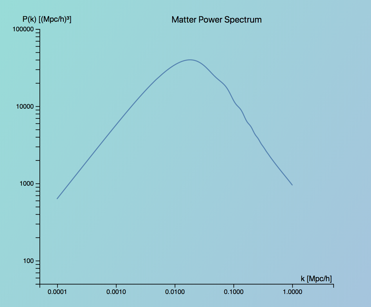
The matter power spectrum - P(k) - describes the large scale structure of the universe - it tells us on which scales matter is distributed. P(k) is a function of wavenumber k which k corresponds to inverse scale - so increasing wavenumber means decreasing scale.
For example, using the visualization, we can see that by increasing the matter content of the universe, we increase the power at large wavenumber, which corresponds to smaller scales. This occurs due to enhanced structure formation as a result of the additional matter content.
CMB Angular Power Spectrum
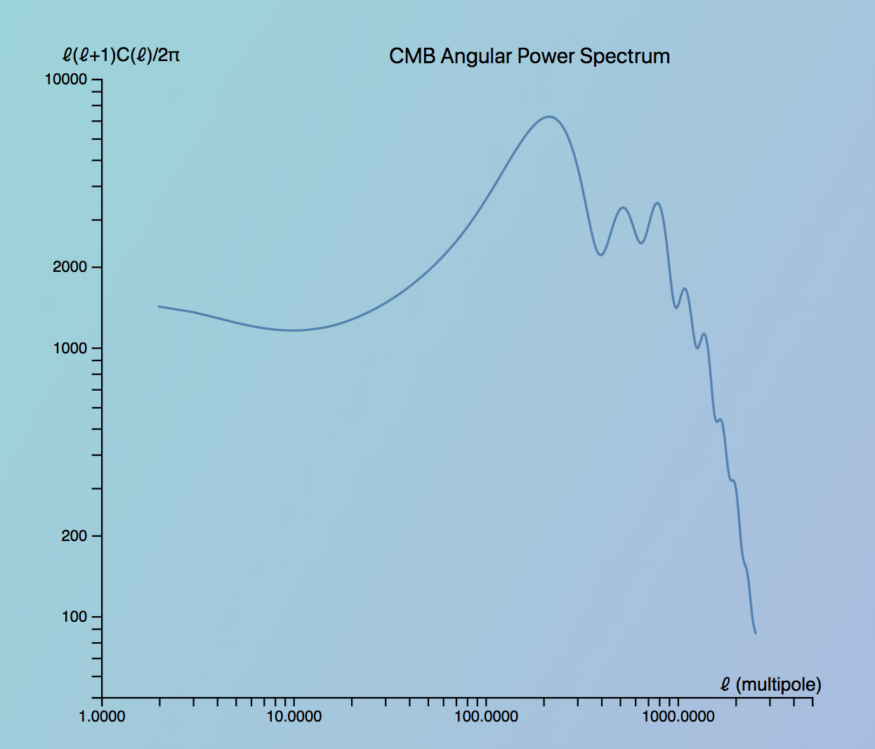
The Cosmic Microwave Background (CMB) radiation was produced only ~100,000 years after the Big Bang, and gives us information about the universe at these early times. One observable from this radiation is the CMB angular power spectrum, which describes anisotropies in the temperature of the CMB radiation as a function of angular scale. Since this temperature anisotropy is defined over a sphere, the temperature anisotropy is separated out into angular scales using a multipole expansion (to read how this multipole expansion is done in detail, check out these notes (PDF)). The spectrum Cℓ (plotted as ℓ(ℓ+1)Cℓ) is a function of multipole ℓ, so increasing multipole corresponds to decreasing angular scales.
Visualizing Power Spectra
Note: This visualization was created in collaboration with Eric Baxter, astrophysics postdoc at UPenn.
To visualize how these power spectra change as a function of cosmological parameters,
we used d3.js, a popular JavaScript library for creating interactive visualizations.
Launch the visualization here!
As the user moves a given slider, the spectra are updated by linearly interpolating between the nearest pre-computed spectra. To create the pre-computed spectra, we used CAMB, a software package for computing power spectra based on input cosmological parameters to generate power and CMB spectra around a fiducial value. We selected a fiducial model from the 2015 results from the Planck Collaboration (PDF). The universe was kept spatially flat (i.e. Ωm + ΩΛ = 1) both because it is a well established constraint and to reduce the amount of data that we needed to generate with CAMB.
If you’d like to check out the code, it’s available here on GitHub. If you’d like to learn more about the effect of cosmological parameters on the power spectra, check out this tutorial.